Examples

Group Lasso with Interaction Terms

import adelie as ad
import numpy as np

In regression settings, we typically want to include pairwise interaction terms amongst a subset of features to capture some non-linearity. Moreover, we would like to perform feature selection on the interaction terms as well. However, to achieve an interpretable model, we would like to also impose a hierarchy such that interaction terms are only included in the model if the main effects are included. Michael Lim and Trevor Hastie provide a formalization of this problem using group lasso where the group structure imposes the hierarchy and the group lasso penalty allows for feature selection. For further details, we provide the following reference:

• Learning interactions via hierarchical group-lasso regularization

We will work under a simulation setting. We draw \(n\) independent samples \(Z_i \in \mathbb{R}^d\) where the continuous features are sampled from a standard normal and the discrete features are sampled uniformly.

n = 1000        # number of samples
d_cont = 10     # number of continuous features
d_disc = 10     # number of discrete features
seed = 1        # random seed

np.random.seed(seed)
Z_cont = np.random.normal(0, 1, (n, d_cont))
levels = np.random.choice(10, d_disc, replace=True) + 1
Z_disc = np.array([np.random.choice(lvl, n, replace=True) for lvl in levels]).T

It is customary to first center and scale the continuous features so that they have mean \(0\) and standard deviation \(1\).

Z_cont_means = np.mean(Z_cont, axis=0)
Z_cont_stds = np.std(Z_cont, axis=0, ddof=0)
Z_cont = (Z_cont - Z_cont_means) / Z_cont_stds

This gives us a combined data matrix \(Z\) with the appropriate levels information. By convention, a \(0\)-level feature is a continuous feature and otherwise it is a discrete feature with that many levels.

Z = np.asfortranarray(np.concatenate([Z_cont, Z_disc], axis=1))
levels = np.concatenate([np.zeros(d_cont), levels])

We generate the response vector \(y\) from a linear model where one continuous and discrete main effects as well as their interaction term are included.

Z_one_hot_0 = np.zeros((n, int(levels[d_cont])))
Z_one_hot_0[np.arange(n), Z_disc[:, 0].astype(int)] = 1
Z_cont_0 = Z_cont[:, 0][:, None]
Z_sub = np.concatenate([
    Z_cont_0,
    Z_one_hot_0,
    Z_cont_0 * Z_one_hot_0,
], axis=1)
beta = np.random.normal(0, 1, Z_sub.shape[1])
y = Z_sub @ beta + np.random.normal(0, 1, n)

We are now in position to construct the full feature matrix to fit a group lasso model. As a demonstration, suppose we (correctly) believe that there is a true interaction term containing the first continuous feature, but we do not know the other feature. We, therefore, wish to construct an interaction between the first continuous feature against all other features. It is easy to specify this pairing, as shown below via intr_map. The following code constructs the interaction matrix X_intr.

intr_map = {
    0: None,
}
X_intr = ad.matrix.interaction(Z, intr_map, levels)

To put all groups of features on the same relative “scale”, we must further center and scale all interaction terms between two continuous features. Then, it can be shown that interactions between two discrete features induce a (Frobenius) norm of \(1\), a discrete and continuous feature induce a norm of \(\sqrt{2}\), and two continuous features induce a norm of \(\sqrt{3}\). These values will be used as penalty factors later when we call the group lasso solver. We first compute the necessary centers and scales.

pairs = X_intr._pairs
pair_levels = levels[pairs]
is_cont_cont = np.prod(pair_levels == 0, axis=1).astype(bool)
cont_cont_pairs = pairs[is_cont_cont]
cont_cont = Z[:, cont_cont_pairs[:, 0]] * Z[:, cont_cont_pairs[:, 1]]
centers = np.zeros(X_intr.shape[1])
scales = np.ones(X_intr.shape[1])
cont_cont_indices = X_intr.groups[is_cont_cont] + 2
centers[cont_cont_indices] = np.mean(cont_cont, axis=0)
scales[cont_cont_indices] = np.std(cont_cont, axis=0, ddof=0)

Now, we construct the full feature matrix \(X\) including the one-hot encoded main effects as well as the standardized version of the interaction terms using the centers and scales defined above.

X_one_hot = ad.matrix.one_hot(Z, levels)
X = ad.matrix.concatenate([
    X_one_hot,
    ad.matrix.standardize(
        X_intr,
        centers=centers,
        scales=scales,
    ),
], axis=1)

Before calling the group lasso solver, we must prepare the grouping and penalty factor information.

groups = np.concatenate([
    X_one_hot.groups,
    X_one_hot.shape[1] + X_intr.groups,
])

is_cont_disc = np.logical_xor(pair_levels[:, 0], pair_levels[:, 1])
penalty = np.ones(X_intr.groups.shape[0])
penalty[is_cont_cont] = np.sqrt(3)
penalty[is_cont_disc] = np.sqrt(2)
penalty = np.concatenate([
    np.ones(X_one_hot.groups.shape[0]),
    penalty,
])

Finally, we call the group lasso solver with our prepared inputs.

state = ad.grpnet(
    X=X,
    glm=ad.glm.gaussian(y),
    groups=groups,
    penalty=penalty,
)

100%|██████████| 100/100 [00:00:00<00:00:00, 4657.95it/s] [dev:71.1%]

First, observe that the first two groups of features that enter the model are precisely the first continuous and discrete main effects.

state.betas[13, :X_one_hot.shape[1]].indices

array([ 0, 10, 11, 12, 13, 14], dtype=int32)

Next, we see that the first interaction terms to be included corresponds to the interaction between the first continuous and discrete features in Z.

first_intr_index = X_one_hot.shape[1] + state.betas[16, X_one_hot.shape[1]:].indices[0]
relative_index = np.argmax(groups == first_intr_index) - X_one_hot.groups.shape[0]
pairs[relative_index]

array([ 0, 10], dtype=int32)

We conclude that the group lasso correctly finds the causal effects of \(y\) early in the path.

Model-X Knockoffs with Lasso Feature Importance Scores

import adelie as ad
import knockpy
import matplotlib.pyplot as plt
import numpy as np

In this example, we cover a neat application of Lasso in a popular statistical method called Knockoffs, pioneered by Rina Barber and Emmanuel Candès. We briefly describe the Knockoff framework. Knockoffs are fictitious features generated by the user that look similar to an already given set of features. As soon as these knockoffs enjoy certain statistical properties relating their distributions to the original features, we may use them to determine which of the original features are important for predicting the response while controlling for the false discovery rate (FDR). For an in-depth treatment of Knockoffs, we provide the following references:

• Panning for Gold: ‘Model-X’ Knockoffs for High Dimensional Controlled Variable Selection

• Papers about Knockoffs

• Knockoffs on Wikipedia

We will work under the Model-X framework. Let’s begin with some data. We assume \(n\) independent samples \(X_i \sim N(0, \Sigma)\) where \(\Sigma \in \mathbb{R}^{p \times p}\) is the equi-correlation matrix with correlation \(\rho\). Our response \(y\) is generated from a linear model \(y = X \beta + \sigma \varepsilon\) where the first half of the coefficients \(\beta\) are generated from \(N(0,1)\) (and the rest set to zero), \(\varepsilon \sim N(0, I_n)\), and \(\sigma\) such that the signal-to-noise ratio is \(1\).

n = 10000       # number of samples
p = 100         # number of features
n_h1 = p // 2   # number of features with signal
rho = 0.3       # equi-correlation
seed = 0        # random seed

np.random.seed(seed)
W = np.random.normal(0, 1, n)
Z = np.random.normal(0, 1, (n, p))
X = np.sqrt(rho) * W[:, None] + np.sqrt(1-rho) * Z
y = X[:, :n_h1] @ np.random.normal(0, 1, n_h1) + np.sqrt(n_h1) * np.random.normal(0, 1, n)

Next, we generate our Model-X knockoffs. The definition of Model-X knockoffs states that each knockoff \(\tilde{X}_i \in \mathbb{R}^{p}\) must satisfy the exchangeability condition that swapping any subset of the features with the respective positions in \(X_i\) preserves the joint distribution of \((X_i, \tilde{X}_i)\), and \(\tilde{X}_i\) must be conditionally independent of the response \(y_i\) given \(X_i\). Under the Gaussian assumption of \(X_i\), it is possible to show that we may then sample \(\tilde{X}_i\) from \(N(\mu_i, V_i)\) where

\[\begin{split}\begin{align*} \mu_i &= X_i - \mathrm{diag}(s) \Sigma^{-1} X_i \\ V_i &= 2 \mathrm{diag}(s) - \mathrm{diag}(s) \Sigma^{-1} \mathrm{diag}(s) \end{align*}\end{split}\]

and \(\mathrm{diag}(s)\) is any non-negative diagonal matrix such that

\[\begin{split}\begin{align*} \begin{bmatrix} \Sigma & \Sigma - \mathrm{diag}(s) \\ \Sigma - \mathrm{diag}(s) & \Sigma \\ \end{bmatrix} \end{align*}\end{split}\]

is positive semi-definite.

Although there are many possible choices of \(s\) that satisfy the conditions above, we use the MVR method in the knockpy package. To make the situation more realistic, we first estimate \(\Sigma\) using the empirical covariance matrix from \(X\), since, in practice, we often do not know the true covariance matrix \(\Sigma\).

Sigma = np.cov(X.T, ddof=0)
S = knockpy.smatrix.compute_smatrix(Sigma, method="mvr", choldate_warning=False)

Next, we sample the knockoffs using the above formula.

Sigma_inv = np.linalg.inv(Sigma)
mu = X - X @ Sigma_inv @ S
V = 2 * S - S @ Sigma_inv @ S

X_knock = mu + np.random.multivariate_normal(np.zeros(p), V, n)

Before using adelie, we convert X and X_knock into column-major matrices since this storage order is more favorable for our solver.

X = np.asfortranarray(X)
X_knock = np.asfortranarray(X_knock)

Once the knockoffs have been constructed, we must construct some feature importance statistic that places an importance score for each original and knockoff feature. This is where the lasso comes in! A common method is solve the lasso problem with the combined feature matrix \((X, \tilde{X})\) and the response \(y\). Then, we choose our feature importance statistic to be the magnitude of the lasso coefficient, that is, scores \(Z_j = |\hat{\beta}_j(\lambda)|\) and \(\tilde{Z}_j = |\hat{\beta}_{j+p}(\lambda)|\) for the original and knockoff features, respectively. Furthermore, the theory also allows the user to run cross-validation to pick the best \(\lambda\) and construct feature importance statistics based on the solution at that \(\lambda\).

To fit lasso, we first need to concatenate \(X\) and \(\tilde{X}\). Although one could concatenate the two matrices into one large dense matrix, we take this opportunity to demonstrate the usage of adelie.matrix.concatenate, which effectively represents the same matrix but does not require any allocation of a new matrix. In practice, we may work in a high-dimensional setting where the number of features is large, in which case, it may be computationally burdensome to construct a concatenated dense matrix.

Xc = ad.matrix.concatenate([X, X_knock], axis=1)

We run a 5-fold cross-validation (CV) lasso under the Gaussian loss using the combined feature matrix and our response.

cv_res = ad.cv_grpnet(
    X=Xc,
    glm=ad.glm.gaussian(y),
    min_ratio=1e-3,
    seed=0,
    intercept=False,
)

100%|██████████| 100/100 [00:00:00<00:00:00, 397.03it/s] [dev:44.7%]
100%|██████████| 100/100 [00:00:00<00:00:00, 415.55it/s] [dev:45.2%]
100%|██████████| 101/101 [00:00:00<00:00:00, 443.93it/s] [dev:44.9%]
100%|██████████| 100/100 [00:00:00<00:00:00, 442.50it/s] [dev:45.5%]
100%|██████████| 101/101 [00:00:00<00:00:00, 421.39it/s] [dev:45.8%]

We can visualize the average CV loss.

cv_res.plot_loss()
plt.show()

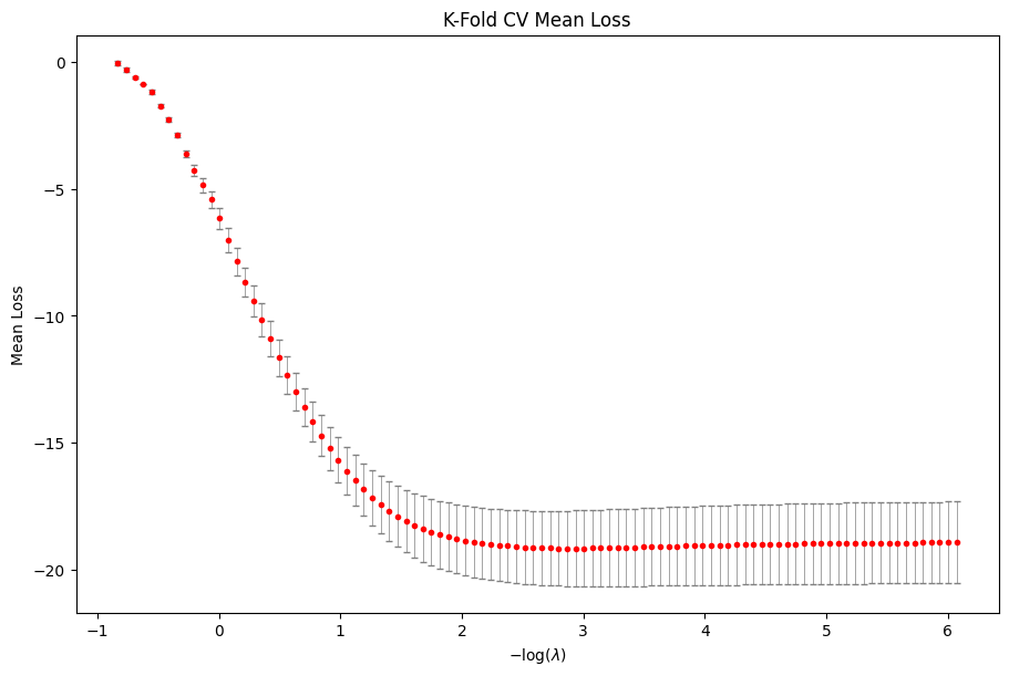
The plot suggests that the best model is somewhere in the middle of the path as the CV loss dips then flattens as we move down the regularization path. We now refit lasso along a regularization path which stops at the best chosen \(\lambda\).

state = cv_res.fit(
    X=Xc,
    glm=ad.glm.gaussian(y),
    intercept=False,
)

100%|██████████| 100/100 [00:00:00<00:00:00, 765.17it/s] [dev:44.4%]

We construct the feature importance statistics by taking the last coefficient vector.

beta = state.betas[-1].toarray()[0]
z = np.abs(beta[:p])
z_knock = np.abs(beta[p:])

Next, we construct the lasso coefficient difference statistics \(W_j = Z_j - \tilde{Z}_j\). A large positive \(W_j\) suggests that the \(j\) th (original) feature is important.

w = z - z_knock

Finally, to control FDR, we apply the Knockoff-filter. For a given level \(q \in [0,1]\), the Knockoff-filter constructs

\[\begin{align*} \tau_+ = \min\{t > 0 : \frac{1 + |\{j : W_j \leq -t\}|}{|\{j : W_j \geq t\}|} \leq q\} \end{align*}\]

and selects features in \(\hat{S} = \{j : W_j \geq \tau_+\}\). This selection procedure controls the FDR so that

\[\begin{align*} \mathbb{E}\left[\frac{|\{j \in \hat{S} \cap \mathcal{H}_0\}|}{|\hat{S}| \vee 1}\right] \leq q \end{align*}\]

where \(\mathcal{H}_0\) is the true set of null features (in this example, \(\mathcal{H}_0 = \{p / 2 + 1,\ldots, p\}\) since the first half of the features is used to construct \(y\)).

We let \(q = 0.05\) in this example and construct \(\tau_+\) using knockpy. We then print the false discovery proportion (FDP), which is the term inside the expectation above, and the power estimate, which is the proportion of correctly selected non-nulls over the total number of non-nulls, or

\[\begin{align*} \widehat{\mathrm{Power}} = \frac{|\hat{S} \cap \mathcal{H}_1|}{|\mathcal{H}_1|} \end{align*}\]

tau_plus = knockpy.knockoff_stats.data_dependent_threshhold(w, 0.05)
S_hat = np.arange(p)[w >= tau_plus]
H0 = np.arange(n_h1, p)
H1 = np.arange(n_h1)
fdp = len(set(S_hat).intersection(set(H0))) / max(S_hat.shape[0], 1)
pwr = len(set(S_hat).intersection(set(H1))) / n_h1
print(f"FDP:    {fdp}")
print(f"Power:  {pwr}")

FDP:    0.11363636363636363
Power:  0.78

For any one experiment, the FDP may not be under \(q\) (though we hope the FDP has a small enough variance that it is not too far from its mean). The guarantee is that if we repeat this entire procedure many times, the average FDP will be under \(q\).

Lasso on GWAS Datasets

import adelie as ad
import matplotlib.pyplot as plt
import numpy as np
import os
import pandas as pd
import pgenlib as pg

In this example, we show how to use adelie to run lasso on GWAS datasets. These datasets often come as .bed or .pgen (PLINK) files accompanied by other files containing metadata. The main feature matrix of interest is the genotype matrix or a single-nucleotide polymorphism (SNP) matrix. This matrix contains values in the range \(\{0,1,2,\mathrm{NA}\}\) with both large number of samples (e.g. 0.5 million) and features (e.g. 1.7 million). As a result, special care must be taken to represent such a large matrix to avoid memory issues and optimize for the matrix operations required to solve the lasso. The response vector is typically some measurement of a phenotype such as standing height. The goal is then to learn the association between the genetic information and the phenotype. We will demonstrate that adelie can easily handle such a use-case.

As a reference, we list a few works in the literature that aim to apply lasso on the UK Biobank, one popular GWAS dataset that has been carefully studied in a wide range of applications.

• A fast and scalable framework for large-scale and ultrahigh-dimensional sparse regression with application to the UK Biobank

• Fast numerical optimization for genome sequencing data in population biobanks

• Fast Lasso method for large-scale and ultrahigh-dimensional Cox model with applications to UK Biobank

• UK Biobank Multi-modality Brain Age LASSO regression analysis

Since we only wish to demonstrate the workflow of using adelie to solve lasso on GWAS datasets, we work with a small-scale example. The example dataset is provided in the data folder, which contains PLINK files for the SNP matrix and a CSV file containing the phenotype and covariates. The PLINK files are taken from SnpArrays.jl. For this demonstration, we randomly generated the phenotype. The covariates include sex and the 10 largest principle components (PCs) of the SNP matrix.

In the following, we outline the steps of applying adelie.

Load the Dense SNP Matrix

The first step is to load the SNP matrix as a dense matrix. We enforce this for two reasons. First, we do not wish to have adelie depend on any particular third-party file formats. This extra dependence complicates the maintenance of the package. Secondly, adelie will save the SNP matrix in its own special format (.snpdat) that is optimized for both memory and speed in some matrix operations required by our solver. Hence, we need to be able to take any user-specified representation of the SNP matrix and convert it into our format. We perform this conversion by first asking the user to read the SNP matrix as a dense matrix then use adelie to convert and save the dense matrix as a .snpdat file.

Due to memory issues, the user should not read the full SNP matrix as a dense matrix! It is recommended to read them in batches of columns instead. Typically, we read per chromosome so that we create 22 .snpdat files.

We now demonstrate using pgenlib how to read the PLINK files as a dense matrix. For more information on how to use pgenlib, we direct the readers to the GitHub page.

We first define the data directory and the relevant PLINK file names.

data_dir = "../../../data"
bedname = os.path.join(data_dir, "EUR_subset.bed")
bimname = os.path.join(data_dir, "EUR_subset.bim")
famname = os.path.join(data_dir, "EUR_subset.fam")

We find the number of samples in the dataset by reading the .fam file. This information is required by pgenlib since we are working with .bed files.

df_fam = pd.read_csv(
    famname,
    sep=" ",
    header=None,
    names=["FID", "IID", "Father", "Mother", "Sex", "Phenotype"],
)
n_samples = df_fam.shape[0]
df_fam

	FID	IID	Father	Mother	Sex	Phenotype
0	1	HG00096	0	0	1	1
1	2	HG00097	0	0	2	1
2	3	HG00099	0	0	2	1
3	4	HG00100	0	0	2	1
4	5	HG00101	0	0	1	1
...	...	...	...	...	...	...
374	375	NA20816	0	0	1	1
375	376	NA20818	0	0	2	1
376	377	NA20819	0	0	2	1
377	378	NA20826	0	0	2	1
378	379	NA20828	0	0	2	1

379 rows × 6 columns

We read the .bim file to retrieve the SNP metadata. We will use this information to read and process the SNP data per chromosome.

df_bim = pd.read_csv(
    bimname,
    sep="\t",
    header=None,
    names=["chr", "variant", "pos", "base", "a1", "a2"],
)
n_snps = df_bim.shape[0]
df_bim

	chr	variant	pos	base	a1	a2
0	17	rs34151105	0.000000	1665	T	C
1	17	rs143500173	0.000000	2748	T	A
2	17	rs113560219	0.000000	4702	T	C
3	17	rs1882989	0.000056	15222	G	A
4	17	rs8069133	0.000499	32311	G	A
...	...	...	...	...	...	...
54046	22	rs113391741	0.750923	51187440	A	G
54047	22	rs151247655	0.750938	51189403	A	G
54048	22	rs187225588	0.751001	51197602	T	A
54049	22	rs9616967	0.751090	51209343	T	A
54050	22	rs148755559	0.751156	51218133	C	T

54051 rows × 6 columns

Let’s try reading the SNP matrix for chromosome 17.

# create bed reader
reader = pg.PgenReader(
    str.encode(bedname),
    raw_sample_ct=n_samples,
)

# get 0-indexed indices for current chromosome
df_bim_chr = df_bim[df_bim["chr"] == 17]
variant_idxs = df_bim_chr.index.to_numpy().astype(np.uint32)

# read the SNP matrix
geno_out_chr = np.empty((variant_idxs.shape[0], n_samples), dtype=np.int8)
reader.read_list(variant_idxs, geno_out_chr)

# convert to sample-major
geno_out_chr = np.asfortranarray(geno_out_chr.T)

Convert to snpdat Format

Now that we have the dense SNP matrix for chromosome 17, we write it in .snpdat format using adelie.

# define cache directory and snpdat filename
cache_dir = "/tmp"
snpdat_name = os.path.join(cache_dir, "EUR_subset_chr17.snpdat")

# create handler to convert the SNP matrix to .snpdat
handler = ad.io.snp_unphased(snpdat_name)
_ = handler.write(geno_out_chr)

That’s it!

Process All Chromosomes

Finally, to mimic the common use-case, we combine all the steps to process all the chromosomes.

We first get a list of the chromosomes in the dataset.

chromosomes = df_bim["chr"].unique()
chromosomes

array([17, 18, 19, 20, 21, 22])

The following code saves each SNP matrix per chromosome as a separate .snpdat file.

# create bed reader
reader = pg.PgenReader(
    str.encode(bedname),
    raw_sample_ct=n_samples,
)

for chr in chromosomes:
    # get 0-indexed indices for current chromosome
    df_bim_chr = df_bim[df_bim["chr"] == chr]
    variant_idxs = df_bim_chr.index.to_numpy().astype(np.uint32)

    # read the SNP matrix
    geno_out = np.empty((variant_idxs.shape[0], n_samples), dtype=np.int8)
    reader.read_list(variant_idxs, geno_out)

    # define snpdat filename
    snpdat_name = os.path.join(cache_dir, f"EUR_subset_chr{chr}.snpdat")

    # create handler to convert the SNP matrix to .snpdat
    handler = ad.io.snp_unphased(snpdat_name)
    _ = handler.write(geno_out_chr)

Load the Feature Matrix

We first load the covariates as a dense matrix and the phenotype as the response vector.

df = pd.read_csv(os.path.join(data_dir, "master_phe.csv"), sep="\t", index_col=0)
covars_dense = df.iloc[:, :-1].to_numpy()
y = df.iloc[:, -1].to_numpy()
df

	sex	PC1	PC2	PC3	PC4	PC5	PC6	PC7	PC8	PC9	PC10	phenotype
0	0	-0.051678	-0.020465	0.046227	-0.014268	0.085271	-0.002017	-0.010386	0.036105	0.010695	-0.082026	4.612085
1	1	-0.050462	0.008577	-0.058172	-0.048560	0.014092	-0.008358	-0.045067	-0.005221	0.098964	0.019094	5.175936
2	1	-0.051158	0.013547	-0.041690	-0.023781	-0.057576	0.088412	0.025772	0.082086	-0.099380	0.016369	13.531050
3	1	-0.051310	-0.021508	0.049910	-0.038484	0.006369	0.001142	0.063346	0.045536	0.021950	-0.019257	188.524040
4	0	-0.051329	0.014914	-0.067042	-0.069162	-0.023286	0.006299	-0.032645	-0.019187	-0.006523	-0.033779	65.697673
...	...	...	...	...	...	...	...	...	...	...	...	...
374	0	-0.051168	-0.048192	0.025948	0.044251	-0.025641	0.000769	0.057611	0.052506	-0.065036	-0.034339	91.516444
375	1	-0.051801	-0.055517	-0.004016	-0.021153	-0.007273	-0.041470	-0.061246	-0.015746	0.020271	0.014094	74.187329
376	1	-0.052525	-0.022246	-0.056309	0.092208	-0.036200	0.070898	-0.010716	0.055041	-0.086128	-0.041673	77.536242
377	1	-0.051577	-0.081801	0.113044	0.024027	0.046088	-0.002275	0.008942	0.020224	0.038375	-0.036612	264.019774
378	1	-0.051611	-0.084751	0.088275	0.026785	0.026810	-0.091582	0.057924	-0.046984	-0.040138	-0.042171	-51.117530

379 rows × 12 columns

Once the SNP matrices have been processed into .snpdat files, we may now load this information as a adelie.matrix.snp_unphased object per file. This matrix class implements certain matrix operations highly efficiently for SNP matrices and is recognized by our solver. Finally, we column-wise concatenate all these matrices as well as the dense covariates.

X = ad.matrix.concatenate(
    [ad.matrix.dense(covars_dense)]
    + [
        ad.matrix.snp_unphased(
            ad.io.snp_unphased(
                os.path.join(cache_dir, f"EUR_subset_chr{chr}.snpdat"),
            )
        )
        for chr in chromosomes
    ],
    axis=1,
)
X.shape

(379, 66257)

Fit Lasso

We fit lasso using X and y under the Gaussian loss with intercept. Note that we unpenalize the covariates.

penalty = np.concatenate([
    np.zeros(covars_dense.shape[-1]),
    np.ones(X.shape[-1] - covars_dense.shape[-1]),
])

state = ad.grpnet(
    X=X,
    glm=ad.glm.gaussian(y),
    penalty=penalty,
)

 44%|████      | 44/100 [00:00:00<00:00:01, 55.52it/s] [dev:90.3%]

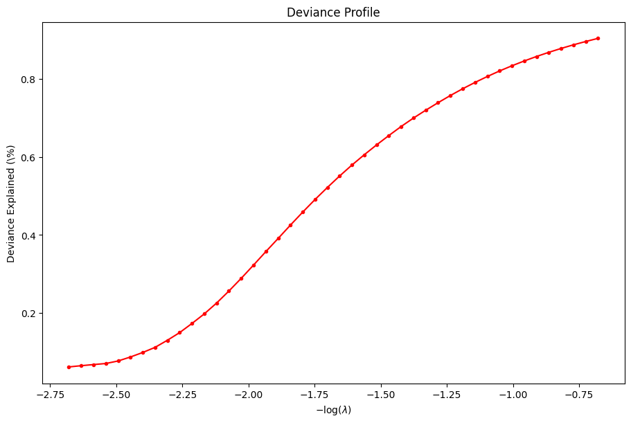
Run Diagnostics (optional)

The user may wish to look at some diagnostic information afterwards. Here is an example of plotting the training \(R^2\).

dg = ad.diagnostic.diagnostic(state)
dg.plot_devs()
plt.show()

Cross-Validation

If the dataset contains few samples, the user may be interested in using cross-validation to determine the best model.

To demonstrate this, we run a 5-fold cross-validation on our dataset.

cv_res = ad.cv_grpnet(
    X=X,
    glm=ad.glm.gaussian(y),
    seed=3,
)

100%|██████████| 102/102 [00:00:01<00:00:00, 61.82it/s] [dev:94.4%]
100%|██████████| 106/106 [00:00:01<00:00:00, 62.96it/s] [dev:94.4%]
100%|██████████| 102/102 [00:00:01<00:00:00, 62.49it/s] [dev:94.7%]
100%|██████████| 100/100 [00:00:01<00:00:00, 64.71it/s] [dev:94.1%]
100%|██████████| 100/100 [00:00:01<00:00:00, 55.79it/s] [dev:93.8%]

We can visualize the average cross-validation loss in the following way.

cv_res.plot_loss()
plt.show()

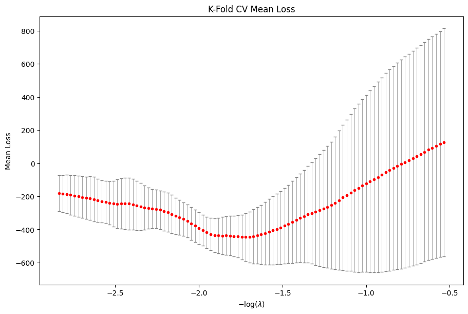
In this example, the best model chosen by 5-fold CV is at index 48 of the \(\lambda\) sequence.

cv_res.best_idx

48

To refit the model at the best model, run the following:

state = cv_res.fit(
    X=X,
    glm=ad.glm.gaussian(y),
)

100%|██████████| 100/100 [00:00:01<00:00:00, 72.60it/s] [dev:51.7%]

The last fitted regularization value is the one corresponding to the best model.

Clean-up Files

Once we are done analyzing the dataset, we may remove the .snpdat files that we created.

for chr in chromosomes:
    os.remove(os.path.join(cache_dir, f"EUR_subset_chr{chr}.snpdat"))

SNP Phased Ancestry

The usual phased calldata is a (n, 2s) matrix of type np.int8 since the entries are one of {0,1} (assuming no missing values), where n is the number of observations and s is the number of SNPs. The factor of 2 comes from the fact that there are always 2 haplotypes. The ancestry information is also a (n, 2s) matrix of type np.int8 where each entry takes on a value in {0,1,..., A-1} where A is the number of ancestry categories. Each ancestry information corresponds to the individual, haplotype, and SNP as in the calldata. We assume that the user has access to a dense matrix of the phased calldata and the corresponding ancestry information prior to using adelie.

The data matrix we ultimately want to use is the sum of the ancestry-expanded calldata for each haplotype, described next. Fix a haplotype, and consider the corresponding calldata and ancestry matrix. For each (i,j) entry of the calldata, suppose it is exanded into a length A vector where a mutation is recorded in entry k if the ancestry at (i,j) is k (and zero otherwise). The concatenation of all these expanded vectors results in (n, As) matrix. Then, we wish to run group lasso by grouping every A columns as a group (i.e. SNP).

To fully mimic the real application, we assume that the calldata is split into chromosomes so that we load column-blocks of the calldata, one chromosome at a time. We will generate n observations and ss[i] SNPs per chromosome for each chromosome i.

n = 1000                        # number of observations
ss = [1000, 2000, 3000]         # number of SNPs per chromosome (3 chromosomes)
A = 8                           # number of ancestries
n_threads = 1                   # number of threads

Similar to the unphased calldata example, we generate our data for each chromosome using a helper function and store a sparse representation in /tmp/spa_chr_i.snpdat for each chromosome i.

filenames = [
    f"/tmp/spa_chr_{i}.snpdat"
    for i in range(len(ss))
]
for i, s in enumerate(ss):
    data = ad.data.snp_phased_ancestry(n, s, A)
    handler = ad.io.snp_phased_ancestry(filenames[i])
    handler.write(data["X"], data["ancestries"], A, n_threads)

We then instantiate our special matrix object for phased ancestry SNP data.

X = ad.matrix.concatenate(
    [
        ad.matrix.snp_phased_ancestry(
            ad.io.snp_phased_ancestry(filename),
            n_threads=n_threads,
        )
        for filename in filenames
    ],
    axis=1,
    n_threads=n_threads,
)

For demonstration purposes, we generate our response vector y from a linear model with only the last three SNPs active in the model.

s = int(np.sum(ss))
p = A * s

np.random.seed(314)
beta = np.random.normal(0, 1, 3*A)
Xb = np.zeros(n)
X.btmul(p-3*A, 3*A, beta, Xb)
y = Xb + np.random.normal(0, 1, n)

Finally, we use adelie to fit group lasso!

state = ad.grpnet(
    X=X,
    glm=ad.glm.gaussian(y=y),
    groups=A * np.arange(s),
    n_threads=n_threads,
)

 62%|██████    | 62/100 [00:00:00<00:00:00, 136.40it/s] [dev:90.5%]

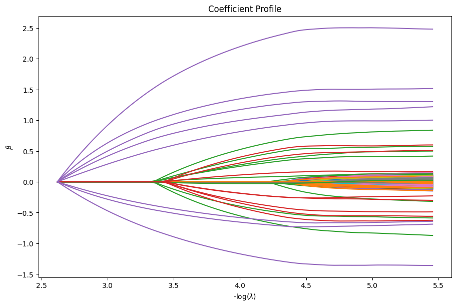
Now, we can use our diagnostic object to inspect our solutions. For example, we can plot the coefficients.

dg = ad.diagnostic.diagnostic(state)
dg.plot_coefficients()
plt.show()

# clean-up generated files!
for filename in filenames: os.remove(filename)