scikit-learn-style API#
In this notebook, we give an overview of using our user-friendly scikit-learn-style API. Oftentimes, existing data analysis pipelines assume scikit-learn API for the models, so it is useful to prepare an adelie solver obeying such an API for seamless integration. Our scikit-learn-style solver is a simple wrapper of the more generic tools provided in adelie. Consequently, it is slightly less flexible (e.g., cannot supply a user-specified GLM). However, it provides many
commonly used functionalities to serve as a quick drop-in replacement for many existing solvers in scikit-learn with adelie.
[1]:
from sklearn.model_selection import train_test_split
from sklearn.metrics import r2_score
from sklearn.datasets import (
    load_breast_cancer,
    load_diabetes,
    load_digits,
)
from sklearn.preprocessing import OneHotEncoder
import adelie as ad
import matplotlib.pyplot as plt
import numpy as np
import scipy.stats as st

np.random.seed(42)
Regression#
We load the diabetes dataset as a regression example and perform a train-test split. Note that we change the storage type for \(X\) to be Fortran-order (column-major) since it is more efficient for our solver.
[2]:
data = load_diabetes()
X, y = data.data, data.target
X_train, X_test, y_train, y_test = train_test_split(X, y, test_size=0.2)
X_train = np.asfortranarray(X_train)
X_test = np.asfortranarray(X_test)
X_train.shape, y_train.shape, X_test.shape, y_test.shape
[2]:
((353, 10), (353,), (89, 10), (89,))
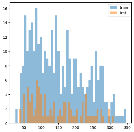
We check that the train and test responses are similar in distribution.
[3]:
f, ax = plt.subplots(1, 1, figsize=(6, 6))
ax.hist(y_train, bins=50, alpha=0.5, label='train')
ax.hist(y_test, bins=50, alpha=0.5, label='test')
ax.legend()
plt.show()

Lasso#
We first instantiate our scikit-learn-style solver class GroupElasticNet. We will use the default setting, which solves the lasso problem with Gaussian loss. As usual, we call fit() with our training data X_train and y_train to solve the lasso along a path of regularization values \(\lambda\).
[4]:
model_gaussian = ad.GroupElasticNet()
model_gaussian.fit(X_train, y_train)
100%|██████████| 100/100 [00:00:00<00:00:00, 2392.51it/s] [dev:52.5%]
[4]:
GroupElasticNet()In a Jupyter environment, please rerun this cell to show the HTML representation or trust the notebook.
On GitHub, the HTML representation is unable to render, please try loading this page with nbviewer.org.
GroupElasticNet()
We call predict() to compute the linear predictions for each \(\lambda\) (each row).
[5]:
yhatmat = model_gaussian.predict(X_test)
yhatmat.shape
[5]:
(100, 89)
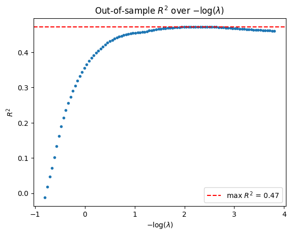
Next, we compute the out-of-sample \(R^2\) for each \(\lambda\) value.
[6]:
r2vec = np.apply_along_axis(lambda yhat: r2_score(y_test, yhat), axis=1, arr=yhatmat)
lam_path = model_gaussian.lambda_
plt.plot(-np.log(lam_path), r2vec, linestyle="None", marker=".")
plt.axhline(r2vec.max(), color="red", linestyle="--", label=f"max $R^2$ = {r2vec.max():.2f}")
plt.title(r"Out-of-sample $R^2$ over $-\log(\lambda)$")
plt.xlabel(r"$-\log(\lambda$)")
plt.ylabel(r"$R^2$")
plt.legend()
plt.show()

K-Fold Cross-Validation#
More often, the user wishes to perform model selection via cross-validation before deploying a model. If the model class is initalized with the "cv_grpnet" solver, we select the best \(\lambda\) by cross-validation and return the model at that \(\lambda\).
[7]:
model_cv_gaussian = ad.GroupElasticNet(solver="cv_grpnet")
model_cv_gaussian.fit(X_train, y_train, min_ratio=1e-3)
100%|██████████| 101/101 [00:00:00<00:00:00, 21478.51it/s] [dev:51.8%]
100%|██████████| 101/101 [00:00:00<00:00:00, 31226.25it/s] [dev:50.8%]
100%|██████████| 101/101 [00:00:00<00:00:00, 39503.28it/s] [dev:57.5%]
100%|██████████| 100/100 [00:00:00<00:00:00, 39044.08it/s] [dev:52.6%]
100%|██████████| 100/100 [00:00:00<00:00:00, 33957.77it/s] [dev:53.0%]
100%|██████████| 100/100 [00:00:00<00:00:00, 43455.42it/s] [dev:52.6%]
[7]:
GroupElasticNet(solver='cv_grpnet')In a Jupyter environment, please rerun this cell to show the HTML representation or trust the notebook.
On GitHub, the HTML representation is unable to render, please try loading this page with nbviewer.org.
GroupElasticNet(solver='cv_grpnet')
With the cv_grpnet backend, calling predict automatically uses the model with the best \(\lambda\).
[8]:
model_cv_gaussian.predict(X_test).shape
[8]:
(89,)
The class also has a score method that computes \(R^2\).
[9]:
model_cv_gaussian.score(X_test, y_test)
[9]:
0.45673736460682524
Binary Classification#
Logistic Regression#
We load the breast_cancer dataset as a binary classification example and perform a train-test split.
[10]:
data = load_breast_cancer()
X, y = data.data, data.target
X_train, X_test, y_train, y_test = train_test_split(X, y, test_size=0.2)
X_train = np.asfortranarray(X_train)
X_test = np.asfortranarray(X_test)
X_train.shape, y_train.shape, X_test.shape, y_test.shape
[10]:
((455, 30), (455,), (114, 30), (114,))
Since we have a binary classification task, we specify our solver to use the "binomial" family for our response. We fit using our cross-validation solver as before.
[11]:
model_cv_binomial = ad.GroupElasticNet(solver="cv_grpnet", family="binomial")
model_cv_binomial.fit(
    X_train,
    y_train.astype(np.float64),
)
100%|██████████| 102/102 [00:00:00<00:00:00, 33514.96it/s] [dev:61.6%]
100%|██████████| 100/100 [00:00:00<00:00:00, 36201.82it/s] [dev:61.8%]
100%|██████████| 101/101 [00:00:00<00:00:00, 42699.36it/s] [dev:64.6%]
100%|██████████| 101/101 [00:00:00<00:00:00, 42445.89it/s] [dev:64.7%]
100%|██████████| 100/100 [00:00:00<00:00:00, 42242.36it/s] [dev:64.2%]
100%|██████████| 100/100 [00:00:00<00:00:00, 41538.31it/s] [dev:63.3%]
[11]:
GroupElasticNet(family='binomial', solver='cv_grpnet')In a Jupyter environment, please rerun this cell to show the HTML representation or trust the notebook.
On GitHub, the HTML representation is unable to render, please try loading this page with nbviewer.org.
GroupElasticNet(family='binomial', solver='cv_grpnet')
For the "binomial" family, the predict method outputs the class label predictions based on the probability estimates. Once we have our class predictions, we can output a contingency table. Here, we see that we never mispredict when the test \(y_i = 1\), but have 16 mispredictions when \(y_i = 0\).
[12]:
yhat = model_cv_binomial.predict(X_test)
st.contingency.crosstab(y_test, yhat).count
[12]:
array([[28, 16],
       [ 0, 70]])
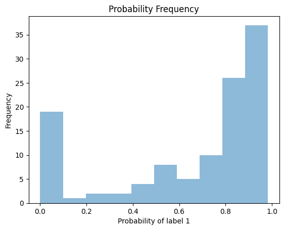
We can compute the probability estimates at the test points and plot the frequency.
[13]:
plt.hist(model_cv_binomial.predict_proba(X_test)[:, 1], alpha = 0.5)
plt.xlabel("Probability of label 1")
plt.ylabel("Frequency")
plt.title("Probability Frequency")
plt.show()

Multi-Class Classification#
Multinomial Regression#
We load the digits dataset as a multi-class classification example and perform a train-test split.
[14]:
data = load_digits()
X, y = data.data, data.target
X_train, X_test, y_train, y_test = train_test_split(X, y, test_size=0.2)
X_train = np.asfortranarray(X_train)
X_test = np.asfortranarray(X_test)
# one-hot-encode labels
oh = OneHotEncoder(sparse_output=False)
y_train2 = oh.fit_transform(y_train[:, np.newaxis])
X_train.shape, y_train.shape, y_train2.shape, X_test.shape, y_test.shape
[14]:
((1437, 64), (1437,), (1437, 10), (360, 64), (360,))
Since we have a multi-class classification task, we specify our solver to use the "multinomial" family for our response. We fit using our cross-validation solver as before.
[18]:
model_cv_multinomial = ad.GroupElasticNet(solver="cv_grpnet", family="multinomial")
model_cv_multinomial.fit(
    X_train,
    y_train2.astype(np.float64),
)
100%|██████████| 100/100 [00:00:01<00:00:00, 75.73it/s] [dev:84.6%]
100%|██████████| 101/101 [00:00:01<00:00:00, 79.43it/s] [dev:84.9%]
100%|██████████| 100/100 [00:00:01<00:00:00, 72.49it/s] [dev:84.8%]
100%|██████████| 101/101 [00:00:01<00:00:00, 75.69it/s] [dev:85.0%]
100%|██████████| 101/101 [00:00:01<00:00:00, 77.03it/s] [dev:85.1%]
100%|██████████| 100/100 [00:00:01<00:00:00, 75.64it/s] [dev:84.7%]
[18]:
GroupElasticNet(family='multinomial', solver='cv_grpnet')In a Jupyter environment, please rerun this cell to show the HTML representation or trust the notebook.
On GitHub, the HTML representation is unable to render, please try loading this page with nbviewer.org.
GroupElasticNet(family='multinomial', solver='cv_grpnet')
For the "multinomial" family, the predict method outputs the class label predictions based on the probability estimates just like the "binomial" family. Once we have our class predictions, we can output a contingency table.
[19]:
yhat = model_cv_multinomial.predict(X_test)
st.contingency.crosstab(y_test, yhat).count
[19]:
array([[29,  0,  0,  0,  0,  0,  0,  0,  0,  0],
       [ 0, 32,  0,  0,  0,  0,  0,  0,  2,  2],
       [ 0,  0, 41,  1,  0,  0,  0,  0,  0,  1],
       [ 0,  1,  0, 34,  0,  0,  0,  0,  1,  0],
       [ 0,  1,  0,  0, 37,  0,  0,  1,  0,  1],
       [ 0,  0,  0,  0,  0, 37,  0,  0,  0,  3],
       [ 0,  1,  0,  0,  0,  0, 37,  0,  0,  0],
       [ 0,  0,  0,  0,  0,  1,  0, 31,  0,  0],
       [ 0,  3,  0,  1,  0,  2,  0,  2, 23,  0],
       [ 0,  0,  0,  0,  0,  0,  0,  1,  0, 34]])